Analyze StrainGE output in Python

Now that we have run StrainGST and StrainGR (including the compare step), how do we analyze the outputs? This page uses Python and its commonly used data science stack (NumPy, SciPy, Pandas and matplotlib+seaborn) to parse the data, plot the relative abundances of strains over time, and generate an ACNI/gap similarity plot.

Download data

We download an archive containing StrainGE outputs part of the vignette described in the paper on the persistence of an E. coli strain in the gut of a woman with recurrent urinary tract infections. The extracted data is organized in a straingst and straingr folder.

!curl --output umb_data.tar.gz https://raw.githubusercontent.com/broadinstitute/strainge-paper/master/umb/umb_data.tar.gz
!tar -xzvf umb_data.tar.gz

  % Total    % Received % Xferd  Average Speed   Time    Time     Time  Current
                                 Dload  Upload   Total   Spent    Left  Speed
100 12196  100 12196    0     0  42347      0 --:--:-- --:--:-- --:--:-- 42347
x straingst/UMB11_01.tsv
x straingst/UMB11_02.tsv
x straingst/UMB11_03.1.tsv
x straingst/UMB11_03.tsv
x straingst/UMB11_04.1.tsv
x straingst/UMB11_04.tsv
x straingst/UMB11_05.tsv
x straingst/UMB11_06.tsv
x straingst/UMB11_07.tsv
x straingst/UMB11_08.tsv
x straingst/UMB11_11.tsv
x straingst/UMB11_12.tsv
x straingr/UMB11_01.tsv
x straingr/UMB11_02.tsv
x straingr/UMB11_03.1.tsv
x straingr/UMB11_03.tsv
x straingr/UMB11_04.1.tsv
x straingr/UMB11_04.tsv
x straingr/UMB11_05.tsv
x straingr/UMB11_06.tsv
x straingr/UMB11_07.tsv
x straingr/UMB11_08.tsv
x straingr/UMB11_11.tsv
x straingr/UMB11_12.tsv
x straingr/compare.summary.chrom.txt

Import required modules

from pathlib import Path

import numpy
import pandas
import matplotlib.pyplot as plt
from IPython.display import display

StrainGST

Read StrainGST outputs and combine it in a DataFrame

The TSV files written by StrainGST contain both sample statistics (the first two lines), and statistics for each identified strain (see StrainGST page). In this tutorial, we are mainly interested in the identified strains. In the code below, when calling pandas.read_csv, we give the argument skiprows=2 to skip the sample statistics.

STRAINGST_DIR = Path("straingst/")

df_list = []
sample_names = []
for f in STRAINGST_DIR.glob("*.tsv"):
    sample_name = f.stem
    df = pandas.read_csv(f, sep='\t', comment='#', skiprows=2, index_col=1)

    df_list.append(df)
    sample_names.append(sample_name)


# Combine all StrainGST results from each sample into a single DataFrame.
straingst_df = pandas.concat(df_list, keys=sample_names, names=["sample"])

sample_names = list(sorted(sample_names, key=lambda e: float(e.replace("UMB11_", ""))))
straingst_df.sort_index()

		i	gkmers	ikmers	skmers	cov	kcov	gcov	acct	even	spec	rapct	old_rapct	wscore	score
sample	strain
UMB11_01	Esch_coli_NGF1	0	49631	49622	50090	0.985	7.009	6.831	0.980	0.987	1.000	1.536	1.505	0.940	0.940
UMB11_02	Esch_coli_NGF1	0	49631	49623	5358	0.103	1.546	0.158	0.932	0.707	1.032	0.048	0.045	0.047	0.048
UMB11_03	Esch_coli_1190	0	48261	48249	37144	0.711	2.814	1.975	0.926	0.826	0.972	0.395	0.366	0.437	0.449
UMB11_03.1	Esch_coli_1190	0	48261	48254	31201	0.595	2.152	1.264	0.918	0.830	1.030	0.711	0.652	0.365	0.376
UMB11_04.1	Esch_coli_1190	0	48261	48250	19042	0.362	1.870	0.668	0.908	0.743	1.047	0.135	0.122	0.173	0.182
UMB11_05	Esch_coli_1190	0	48261	48248	40411	0.775	2.741	2.097	0.923	0.884	0.967	0.484	0.447	0.540	0.558
UMB11_06	Esch_coli_1190	1	48261	21600	30714	0.794	7.102	5.565	0.283	0.797	0.552	1.005	0.391	0.079	0.142
	Esch_coli_H3	0	45610	45560	74449	0.960	114.343	109.038	0.921	0.960	0.976	16.420	16.042	0.795	0.814
UMB11_07	Esch_coli_1190	0	48261	48237	58276	0.854	4.557	3.846	0.803	0.873	0.794	0.411	0.822	0.415	0.522
	Esch_coli_f974b26a-5e81-11e8-bf7f-3c4a9275d6c8	1	47727	21265	17074	0.441	2.588	1.077	0.526	0.668	1.012	0.613	0.106	0.102	0.103
UMB11_08	Esch_coli_1190	0	48261	48248	31599	0.592	2.243	1.309	0.904	0.810	0.980	0.315	0.285	0.344	0.351
UMB11_11	Esch_coli_1190	0	48261	48248	49462	0.920	6.107	5.545	0.920	0.923	0.965	1.180	1.086	0.696	0.721
UMB11_12	Esch_coli_1190	0	48261	48235	66509	0.941	9.061	8.431	0.800	0.941	0.734	0.978	2.020	0.489	0.667
	Esch_coli_26561	1	46249	19738	21112	0.853	4.773	3.983	0.780	0.869	0.968	1.548	0.395	0.486	0.502

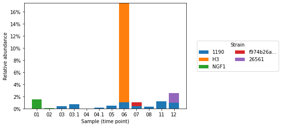
Plot relative abundances

plt.figure(figsize=(6, 4))

strain_order = ['Esch_coli_1190', 'Esch_coli_H3', 'Esch_coli_NGF1', 'Esch_coli_f974b26a-5e81-11e8-bf7f-3c4a9275d6c8', "Esch_coli_26561"]
strain_labels = ['1190', 'H3', 'NGF1', 'f974b26a...', "26561"]
xlabels = [s.replace("UMB11_", "") for s in sample_names]

x = numpy.arange(len(sample_names))
bottom = numpy.zeros((len(sample_names),))
for ref, label in zip(strain_order, strain_labels):
    # Create an array with all relative abundances for the current reference in each sample. If not available, set to zero.
    rel_abun = numpy.array([
        straingst_df.loc[(sample, ref), 'rapct'] if (sample, ref) in straingst_df.index else 0.0
        for sample in sample_names
    ])

    plt.bar(x, rel_abun, bottom=bottom, tick_label=xlabels, label=label, width=0.8)
    bottom += rel_abun

plt.xlabel("Sample (time point)")
plt.ylabel("Relative abundance")
plt.gca().yaxis.set_major_formatter("{x:g}%")
plt.legend(title="Strain", loc="center left", bbox_to_anchor=(1.05, 0.5), ncol=2)

plt.show()

StrainGR

Load call data in a DataFrame

To load StrainGR outputs, we use a similar approach as descried above. In this case, the StrainGR TSV files can be directly loaded with pandas without skiprows.

One thing to note, StrainGR outputs metrics for every contig in the concatenated reference used for alignment. The output file thus contains metrics for contigs from strains that were not predicted to be present by StrainGST. We use the presence/absence predictions of StrainGST as our “truth” and remove the contigs from strains that weren’t present.

We apply a few other filters, including removing plasmid contigs, and contigs with less coverage than 0.5x.

STRAINGR_DIR = Path("straingr/")

df_list = []
sample_names = []
for f in STRAINGR_DIR.glob("*.tsv"):
    df = pandas.read_csv(f, sep='\t', index_col=0)
    df = df.drop(index='TOTAL')  # Remove TOTAL statistics

    df_list.append(df)
    sample_names.append(f.stem)

straingr_df = pandas.concat(df_list, keys=sample_names, names=["sample"])
straingr_df['straingst_present'] = straingr_df.index.map(lambda ix: ix in straingst_df.index)
straingr_df['is_plasmid'] = straingr_df['length'] < 4e6
straingr_df['enough_cov'] = straingr_df['coverage'] > 0.5

# Filter and re-index
straingr_df = straingr_df[straingr_df['straingst_present'] & ~straingr_df['is_plasmid'] & straingr_df['enough_cov']].reset_index().set_index(['sample', 'ref'])
straingr_df

		name	length	coverage	uReads	abundance	median	callable	callablePct	confirmed	confirmedPct	...	multiPct	lowmq	lowmqPct	high	highPct	gapCount	gapLength	straingst_present	is_plasmid	enough_cov
sample	ref
UMB11_11	Esch_coli_1190	NZ_CP023386.1	4900891	2.492	106232	0.449	2	2819899	57.538	2818902	99.965	...	0.004	435239	8.881	488	0.010	9	165998	True	False	True
UMB11_06	Esch_coli_H3	NZ_CP010167.1	4630919	47.519	1331869	7.902	48	3863102	83.420	3861892	99.969	...	0.004	1439048	31.075	84996	1.835	9	120001	True	False	True
	Esch_coli_1190	NZ_CP023386.1	4900891	1.963	69465	0.264	2	1515111	30.915	1513886	99.919	...	0.015	1161951	23.709	699045	14.264	9	165099	True	False	True
UMB11_07	Esch_coli_f974b26a-5e81-11e8-bf7f-3c4a9275d6c8	NZ_LR536430.1	4975029	0.700	14686	0.132	0	378975	7.618	377743	99.675	...	0.013	495996	9.970	17165	0.345	17	347002	True	False	True
	Esch_coli_1190	NZ_CP023386.1	4900891	1.591	59112	0.347	1	1894740	38.661	1893628	99.941	...	0.010	323110	6.593	3384	0.069	12	171056	True	False	True
UMB11_03	Esch_coli_1190	NZ_CP023386.1	4900891	0.822	35131	0.143	1	859998	17.548	859671	99.962	...	0.001	160054	3.266	26	0.001	9	185085	True	False	True
UMB11_01	Esch_coli_NGF1	NZ_CP016007.1	5026105	3.549	85824	0.823	3	2506998	49.880	2506921	99.997	...	0.003	1668501	33.197	3681	0.073	1	16868	True	False	True
UMB11_03.1	Esch_coli_1190	NZ_CP023386.1	4900891	0.596	24708	0.278	0	547015	11.162	546816	99.964	...	0.001	99001	2.020	114	0.002	7	172806	True	False	True
UMB11_08	Esch_coli_1190	NZ_CP023386.1	4900891	0.580	24145	0.118	0	505713	10.319	505494	99.957	...	0.001	115822	2.363	64	0.001	6	158445	True	False	True

9 rows × 23 columns

Load compare data in a DataFrame

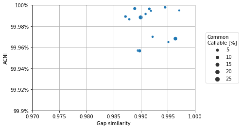
The above data mainly contains data per sample of individual strains as compared to its closest reference. In general, we are often more interested how strains in each sample relate to each other. These kind of relationships are computed with the straingr compare command. Here, we load the data from compare, make sure we only include comparisons between strains that were predicted to be present by StrainGST, and plot the ACNI/gap similarity.

compare_df = pandas.read_csv(STRAINGR_DIR / "compare.summary.chrom.txt", sep='\t', index_col=[0, 1, 2])

def both_straingst_present(ix):
    sample1, sample2, ref = ix

    return (sample1, ref) in straingr_df.index and (sample2, ref) in straingr_df.index

compare_df['both_present'] = compare_df.index.map(both_straingst_present)
compare_df = compare_df[compare_df['both_present']].copy()
compare_df

			scaffold	length	common	commonPct	single	singlePct	singleAgree	singleAgreePct	sharedAlleles	sharedAllelesPct	...	BnotAweak	BnotAweakPct	Agaps	AsharedGaps	AgapPct	Bgaps	BsharedGaps	BgapPct	gapJaccardSim	both_present
sample1	sample2	ref
UMB11_03	UMB11_03.1	Esch_coli_1190	NZ_CP023386.1	4900891	126732	2.5859	126732	100.0000	126725	99.9945	126725	99.9945	...	5	17.8571	185085	163905	88.5566	172806	172806	100.0000	0.9919	True
	UMB11_06	Esch_coli_1190	NZ_CP023386.1	4900891	336010	6.8561	335954	99.9833	335809	99.9568	335865	99.9568	...	160	57.3477	185085	163905	88.5566	165099	158136	95.7825	0.9895	True
	UMB11_07	Esch_coli_1190	NZ_CP023386.1	4900891	405110	8.2660	405067	99.9894	405023	99.9891	405066	99.9891	...	65	32.5000	185085	175075	94.5917	171056	154895	90.5522	0.9872	True
	UMB11_08	Esch_coli_1190	NZ_CP023386.1	4900891	117635	2.4003	117635	100.0000	117629	99.9949	117629	99.9949	...	2	3.8462	185085	145541	78.6347	158445	146928	92.7312	0.9971	True
	UMB11_11	Esch_coli_1190	NZ_CP023386.1	4900891	611275	12.4727	611224	99.9917	611203	99.9966	611254	99.9966	...	29	11.9835	185085	185085	100.0000	165998	165998	100.0000	0.9889	True
UMB11_03.1	UMB11_06	Esch_coli_1190	NZ_CP023386.1	4900891	215863	4.4046	215823	99.9815	215758	99.9699	215798	99.9699	...	95	71.4286	172806	172806	100.0000	165099	158136	95.7825	0.9922	True
	UMB11_07	Esch_coli_1190	NZ_CP023386.1	4900891	252557	5.1533	252524	99.9869	252490	99.9865	252523	99.9865	...	56	43.0769	172806	172806	100.0000	171056	148033	86.5407	0.9879	True
	UMB11_08	Esch_coli_1190	NZ_CP023386.1	4900891	75899	1.5487	75897	99.9974	75894	99.9960	75896	99.9960	...	2	10.0000	172806	148091	85.6978	158445	146928	92.7312	0.9916	True
	UMB11_11	Esch_coli_1190	NZ_CP023386.1	4900891	390913	7.9764	390894	99.9951	390880	99.9964	390899	99.9964	...	14	14.0000	172806	172806	100.0000	165998	154893	93.3102	0.9916	True
UMB11_06	UMB11_07	Esch_coli_1190	NZ_CP023386.1	4900891	718395	14.6585	718228	99.9768	717916	99.9566	718083	99.9566	...	151	22.1083	165099	158136	95.7825	171056	148033	86.5407	0.9898	True
	UMB11_08	Esch_coli_1190	NZ_CP023386.1	4900891	199668	4.0741	199626	99.9790	199556	99.9649	199598	99.9649	...	18	11.1111	165099	151355	91.6753	158445	158445	100.0000	0.9951	True
	UMB11_11	Esch_coli_1190	NZ_CP023386.1	4900891	1059446	21.6174	1059249	99.9814	1058911	99.9681	1059108	99.9681	...	50	6.2500	165099	158136	95.7825	165998	154893	93.3102	0.9964	True
UMB11_07	UMB11_08	Esch_coli_1190	NZ_CP023386.1	4900891	235328	4.8017	235291	99.9843	235271	99.9915	235308	99.9915	...	6	5.1724	171056	131119	76.6527	158445	146928	92.7312	0.9909	True
	UMB11_11	Esch_coli_1190	NZ_CP023386.1	4900891	1284089	26.2011	1283913	99.9863	1283763	99.9883	1283939	99.9883	...	26	3.8981	171056	154895	90.5522	165998	160523	96.7018	0.9900	True
UMB11_08	UMB11_11	Esch_coli_1190	NZ_CP023386.1	4900891	358765	7.3204	358752	99.9964	358744	99.9978	358757	99.9978	...	5	3.6765	158445	146928	92.7312	165998	139943	84.3040	0.9945	True

15 rows × 32 columns

import seaborn

seaborn.scatterplot(x="gapJaccardSim", y="singleAgreePct", size="commonPct", data=compare_df)

plt.xlim(0.970, 1.0)
plt.xlabel("Gap similarity")

plt.ylim(99.9, 100)
plt.ylabel("ACNI")
plt.gca().yaxis.set_major_formatter("{x:g}%")

plt.grid('on')
plt.legend(title="Common\nCallable [%]", loc="center left", bbox_to_anchor=(1.05, 0.5))

<matplotlib.legend.Legend at 0x160142700>